11 — Decision Science: MDP sequencing + SHAP-style explainability
The brief's hint resources — Markov Decision Process and SHAP decision plots — signal that the "automated workflow" should be quantitatively rigorous and explainable, not a black box. This doc shows how both are now wired into MarketPulse, and what they tell us. Runnable code:
decision-science/.
Were they used before? Not explicitly — now they are.
Our market-entry engine was already a sequential decision under uncertainty (Wave 1→2→3) with a weighted scoring model. We formalize the first as an MDP and make the second explainable with exact Shapley values. Both validate (and stress-test) the recommended strategy.
A. SHAP-style explainability of the market score
The attractiveness score is an additive weighted model: score(m) = Σ wᵢ · xᵢ(m). For
additive models the Shapley value is exact and closed-form:
φᵢ(m) = wᵢ · ( xᵢ(m) − mean_i ) and score(m) = base + Σ φᵢ(m), base = Σ wᵢ·mean_i
So we get a genuine SHAP decomposition without the shap library — and we can say so, which is itself a sophistication point. Outputs:
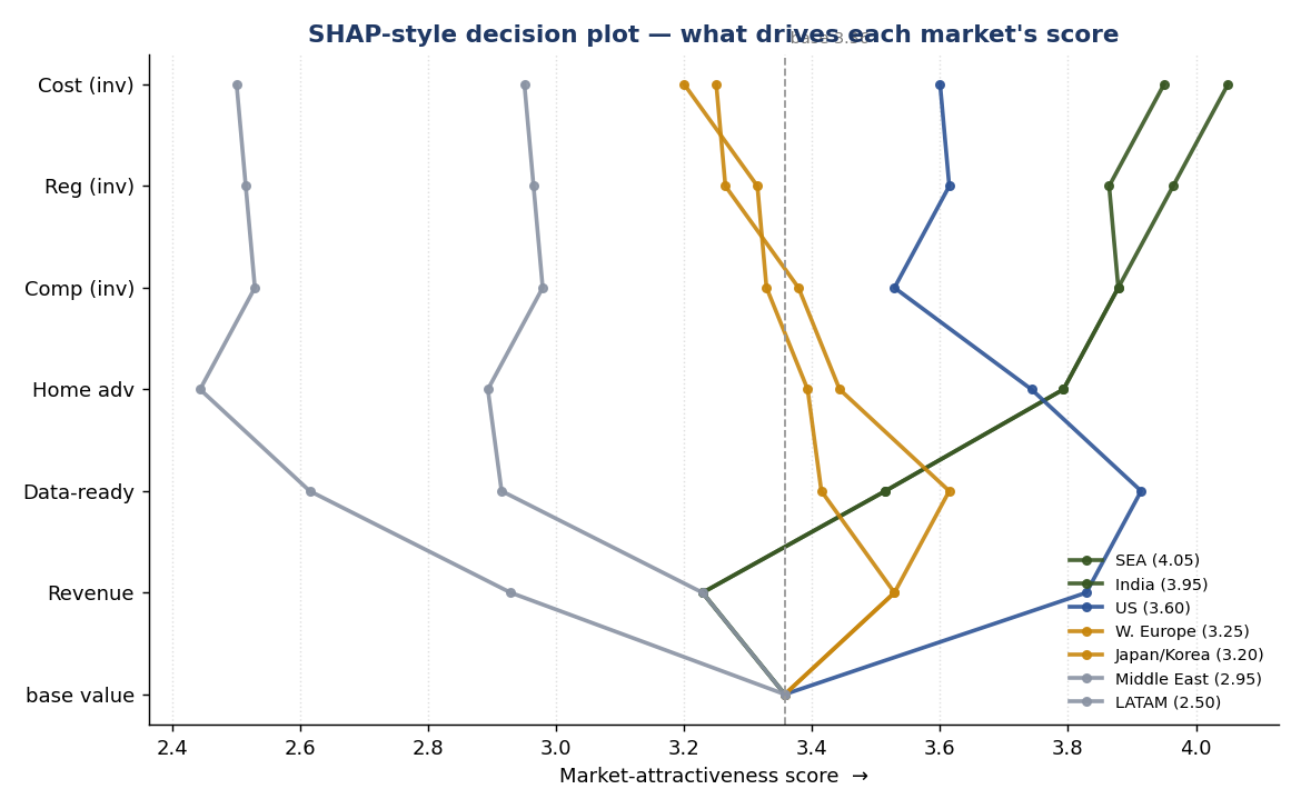
assets/decision_plot.png— SHAP-style decision plot: each market is a line rising from the base value, bending left/right as each criterion adds/subtracts, ending at its final score.decision-science/outputs/waterfall_*.png— per-market waterfalls (what pushes a market up vs. down).decision-science/outputs/shap_contributions.csv— the exact numbers.
What it reveals: US is dragged from the top by Home-advantage and Competition despite the strongest Revenue contribution; SEA/India win on Data-readiness + Home-advantage. This is exactly why the blended score ranks SEA/India above the US — now transparent, not asserted.
B. Market entry as a Markov Decision Process
We model sequencing formally:
| MDP element | MarketPulse meaning |
|---|---|
| State | (period t, set of markets already established) |
| Action | attempt to enter one not-yet-entered market (or wait) |
| Transition | attempt succeeds with prob pₘ (uncertainty); reuse synergies lower cost (US compliance → W. Europe; Japan partner model → Middle East) |
| Reward | expected discounted recurring ARR − entry cost |
| Policy | the optimal entry order, from value iteration (backward induction) |
Solved two ways (decision-science/mdp_sequencing.py):
- Scenario A — naïve (risk-neutral): optimal order = US → W. Europe → Japan/Korea → SEA → India (V₀ ≈ $16.1M). A pure expected-value model says "go where the money is, first."
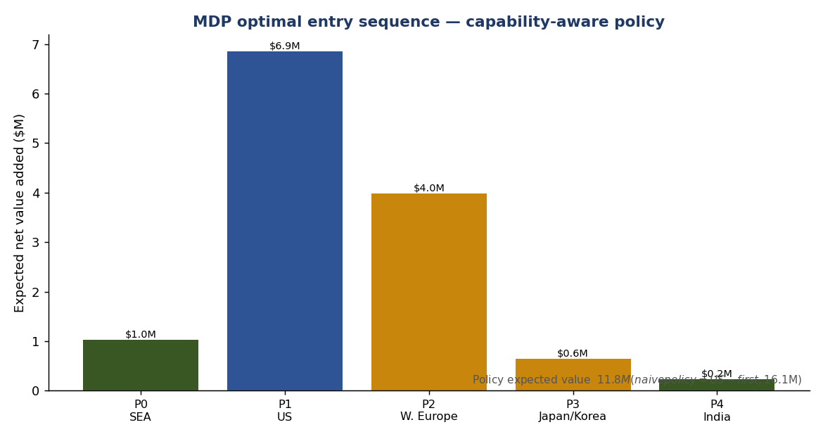
- Scenario B — capability-aware [recommended]: apply a cold-start penalty — entering a hard market (US/EU/Japan) with no reference logos or proven local motion yet is much riskier. Optimal order flips to SEA → US → W. Europe → Japan/Korea → India (V₀ ≈ $11.8M).
The insight (this is the valuable part)
The naïve MDP rushes the US; the moment you price in the real risk of going cold (no
references, unproven sales motion, capital concentration), the optimum lands a cheap home win
first, then attacks the US — precisely the Wave-1-then-US logic in 07.
So the MDP doesn't just decorate the strategy; it explains why deepening SEA/India first is
risk-adjusted-optimal, and it quantifies the cost of getting sequencing wrong (~$4M of expected
value swings on the cold-start assumption alone — a number worth de-risking with references).
How this upgrades the automated engine
The engine in workflow/market-entry-automation.md gets two
rigorous cores: (1) the SHAP decomposition makes step-2 Score explainable to stakeholders;
(2) the MDP makes step-3 Decide an optimal policy under uncertainty, not a static rule —
re-solve as pₘ, costs, or synergies change.
Run it
cd decision-science
pip install -r requirements.txt
python explain_scores.py     # SHAP-style plots + CSV
python mdp_sequencing.py     # MDP scenarios A & B + chart
Caveats (intellectual honesty)
All pₘ, values, costs and the cold-start penalty are illustrative, benchmark-anchored
assumptions (Ai Palette is private). The point is the method and the sensitivity, not the
decimal places — change the inputs and the policy updates.